Optimizing GPU Usage

Exam guide§2.1

Modern AI training demands immense resources, and even small inefficiencies inflate cost and slow progress. This page introduces ML Productivity Goodput - a metric for the true efficiency of an AI training job - then walks through the decision trees for picking the right GPU and squeezing the most performance per dollar out of it.

ML Productivity Goodput

In networking, goodput measures application-level throughput. In ML training it means the same thing in spirit: not how much data the GPUs process, but how much effective training progress you make. The goodput ratio (usually just "goodput") is a unitless percentage - effective training progress divided by total potential throughput - an easy-to-read indicator of training efficiency.

Goodput ratio - effective training progress as a fraction of total throughput. A 60% goodput means 40% of the potential compute produced no training progress.

⚠GotchaFailure cost scales quadratically

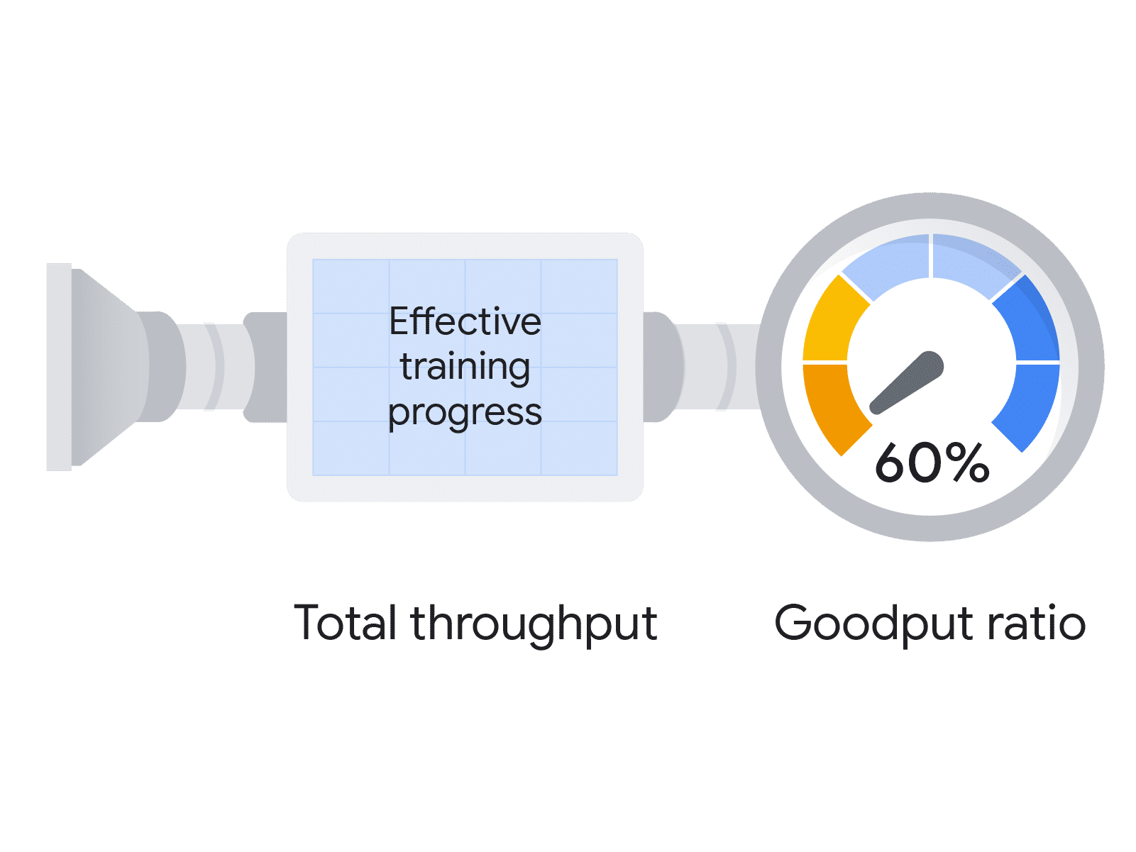
For large-scale training on massive clusters, the cost of failure rises quadratically with scale. That makes understanding and maximizing goodput critical to the viability of big AI projects - not a nice-to-have.

ML Productivity Goodput is the product of three metrics:

ML Productivity Goodput = Scheduling goodput x Runtime goodput x Program goodput.

≡FactsThe three goodput metrics

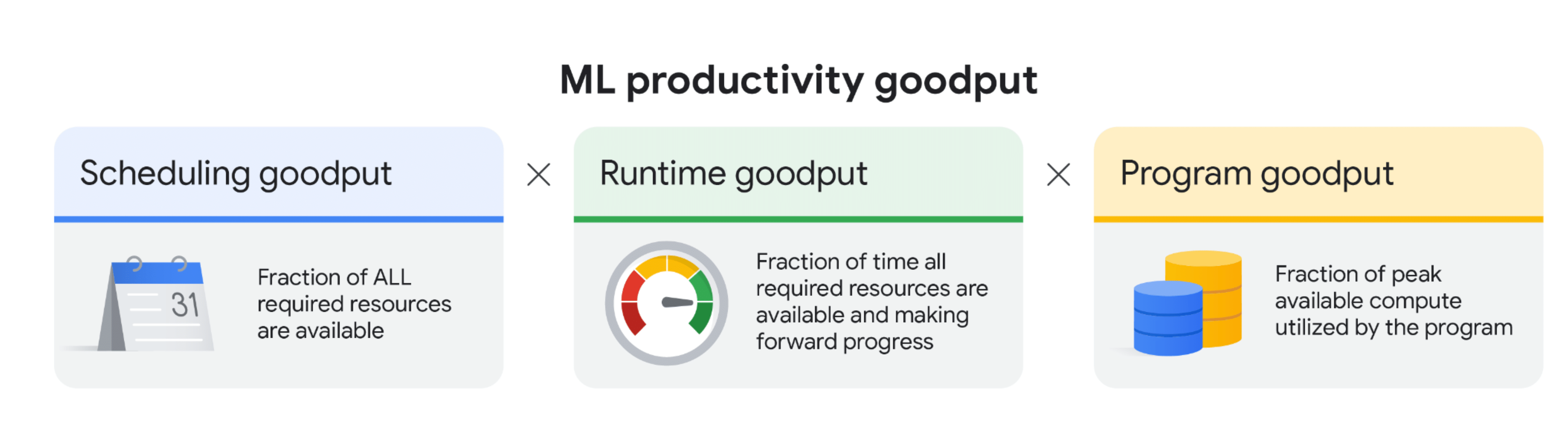
• Scheduling goodput - the fraction of time that all resources the job needs are actually available. On-demand or preemptible instances can hit stockouts, which drags this down.
• Runtime goodput - the fraction of available time spent making forward progress. Interruptions and slow resumes erode it.
• Program goodput - also called model FLOP utilization (MFU): the fraction of the hardware's peak performance the job actually extracts.

AI Hypercomputer - Google's supercomputing architecture - is designed around these metrics, with capabilities at each layer that target a specific goodput.

AI Hypercomputer layers map to goodput: flexible consumption (DWS, on-demand, CUD, Spot) drives scheduling goodput; libraries and frameworks drive program goodput; GKE and Compute Engine drive runtime goodput.

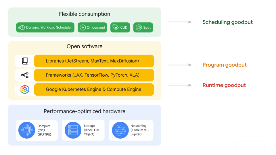
Scheduling goodput

Scheduling goodput is about keeping every required resource available for the whole run. Two techniques help:

Technique	What it does
Resource reservation	For short-term usage, reserve compute up front (for example with DWS calendar mode) to ensure consistent availability and avoid stockouts. DWS flex mode starts the job only once all required resources are available.
Hot spares	Keep pre-provisioned, idle resources ready to take over, minimizing the time to schedule resources when resuming from an interruption.

Runtime goodput

The core of runtime goodput is the number of useful training steps completed over a period. You can estimate it with an analytical model built on the cost of each interruption.

Runtime goodput timeline - between the last checkpoint and the reschedule, badput accumulates as t_ch (progress lost since the last checkpoint) plus t_rm (time to resume).

≡FactsRuntime goodput model

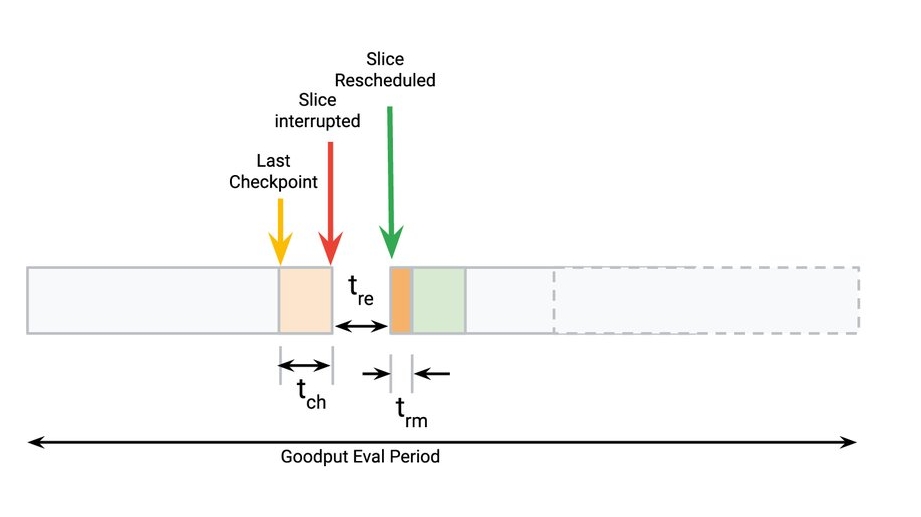
• t_ch - time since the last checkpoint when a failure occurs.
• t_rm - time to resume training after an interruption.
• t_re - time to reschedule the slice.
• t_w - goodput eval period.
• N - number of interruptions.
• Cost of interruption (badput): t_c = ΣN (t_rm + t_ch)
• Runtime goodput = (t_w - t_c - ΣN·t_re) / (t_w - ΣN·t_re)

To maximize runtime goodput, minimize t_ch and t_rm. (The reschedule time t_re matters too, but it is accounted for under scheduling goodput.) Two recommended methods:

Method	How it helps
Enable auto-checkpointing	The job triggers a checkpoint on a SIGTERM signal that warns of imminent interruption (defrag preemption, maintenance), cutting progress lost since the last checkpoint - it minimizes t_ch. Available in tools like Orbax and MaxText.
Use container pre-loading	On GKE, preload containers and models from a secondary boot disk so images are available almost instantly when a failed node returns - minimizing t_rm. Preloading a 16 GB container is about 29x faster than pulling from a container registry.

Program goodput (MFU)

Program goodput - model FLOP utilization - is how efficiently the program uses the GPU hardware. It is shaped by the distribution strategy, how well compute and communication overlap, memory-access efficiency, and pipeline design. The XLA compiler (a core AI Hypercomputer component) helps maximize it with out-of-the-box optimizations and scalable APIs like GSPMD. Key techniques:

Technique	What it does
Custom kernels with XLA (Jax/Pallas)	An escape hatch to hand-write kernels for complex computation blocks on Cloud TPUs and GPUs (Jax and PyTorch/XLA). Examples like flash attention or block-sparse kernels significantly improve program goodput at larger sequence lengths.
Host offload	Accelerator memory is limited. Offload activations from the forward pass to host DRAM and reuse them in the backward pass for gradient computation, saving recomputation cycles.
Int8 mixed-precision (AQT)	Accurately Quantized Training maps a subset of matrix multiplications to 8-bit integers to boost efficiency without compromising model convergence.

Choosing the right GPU

A GPU decision tree gives a structured way to pick hardware for a workload. The very first branch is always the same: is the workload training/fine-tuning or inferencing?

Workload	What it is	Demands
Training / fine-tuning	Teaching a model new patterns, or adapting an existing model to specific data.	Compute-intensive, memory-hungry, runs for extended periods.
Inferencing	Applying a pre-trained model to new data to make predictions.	Less compute than training, but often needs high throughput and low latency for real-time use.

GPU decision tree - branch on training vs inferencing, then on scale (VMs / GPU count) and latency to reach a recommendation. Blue ovals are decisions; yellow boxes are recommendations.

?DECISIONWhich GPU for training or fine-tuning?

Single VM or small models→T4 or L4 - efficient, cost-effective; always validate on your actual model and dataset

Distributed, up to 4 VMs / 32 GPUs, latency not critical→L4 - good balance of performance and efficiency (max 32 GPUs or 4 nodes)

Distributed, more than 4 VMs / 32 GPUs, or latency critical→NVLink options (H100, A100, even V100) - high-bandwidth, low-latency interconnect for multi-GPU training at scale

Transformer-based large model (BERT, GPT, other LLMs)→NVLink options (H100, A100, even V100) - high VRAM plus fast inter-GPU communication

Pick this when: T4/L4 for single-VM or small models; L4 up to 32 GPUs / 4 nodes when latency is not critical; NVLink options for very large or latency-critical or transformer LLM training

?DECISIONWhich GPU for inferencing?

Single-GPU inference→T4 or L4 - good cost/performance for single-GPU throughput; validate for your scenario

Multi-GPU within a single VM→T4/L4 recommendation often extends here if performance validates

Distributed, up to 4 VMs / 32 GPUs, latency not critical→L4 - scales moderately (max 32 GPUs or 4 nodes)

Distributed, more than 4 VMs / 32 GPUs, or latency critical→NVLink options (H100, A100, even V100) - bandwidth and low latency for high-throughput, strict-response-time inference

Pick this when: T4/L4 for single-GPU or single-VM multi-GPU; L4 up to 32 GPUs / 4 nodes when latency is not critical; NVLink options for massive scale or every-millisecond latency

⚠GotchaAlways validate on your workload

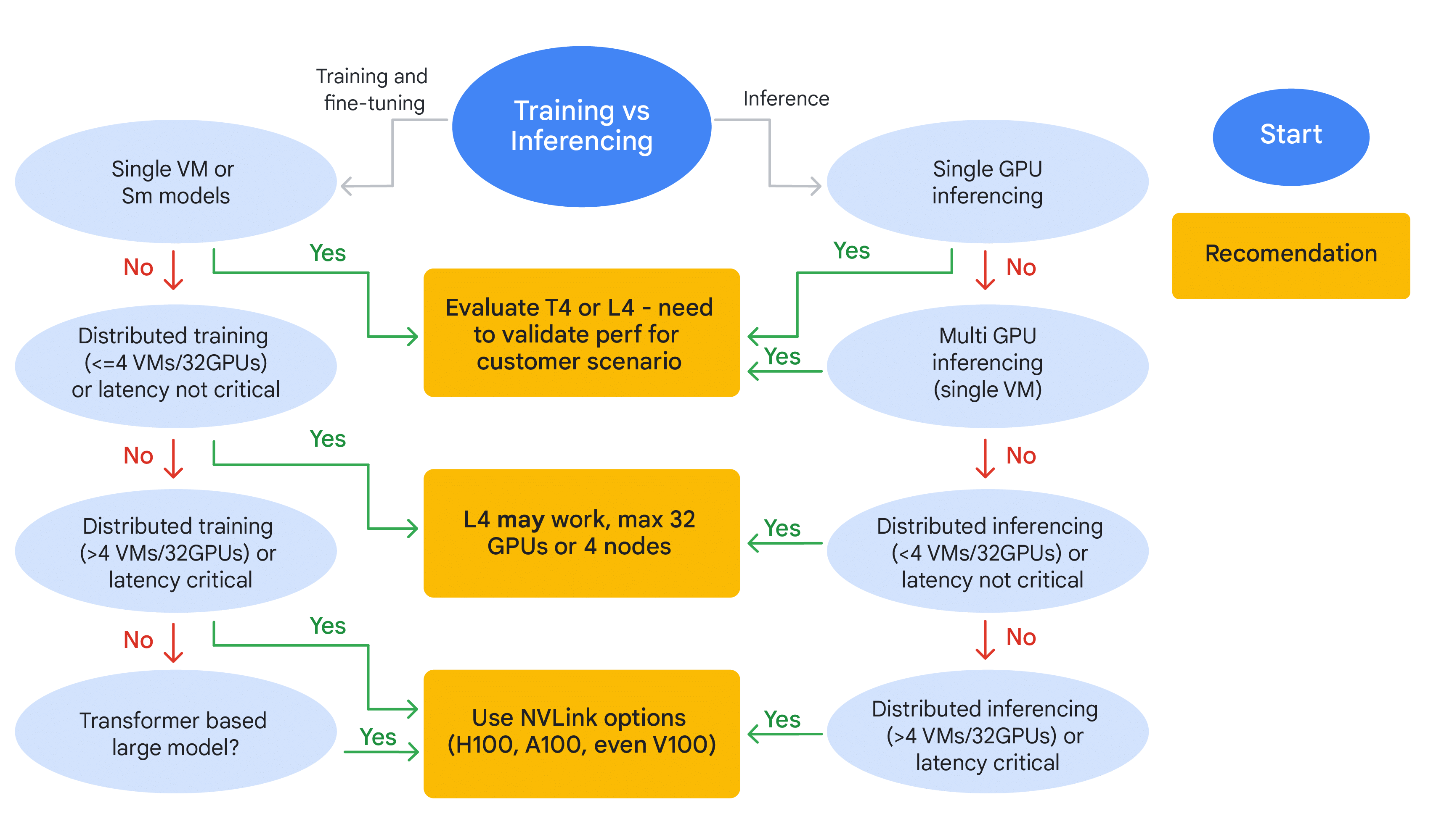
Every recommendation above assumes you confirm it with practical testing on your actual model and dataset. Theoretical fit is a starting point, not a guarantee - especially for the T4/L4 tier.

Optimizing cost and efficiency

Once you are on A100-or-higher GPUs, this tree trims cost by right-sizing to the bottleneck.

Cost and efficiency decision tree - start by finding the bottleneck, right-size down to T4/L4 or smaller shapes where the A100's full power is not needed, then reserve once fast enough or migrate to TPU if not.

#NumbersCost and efficiency flow

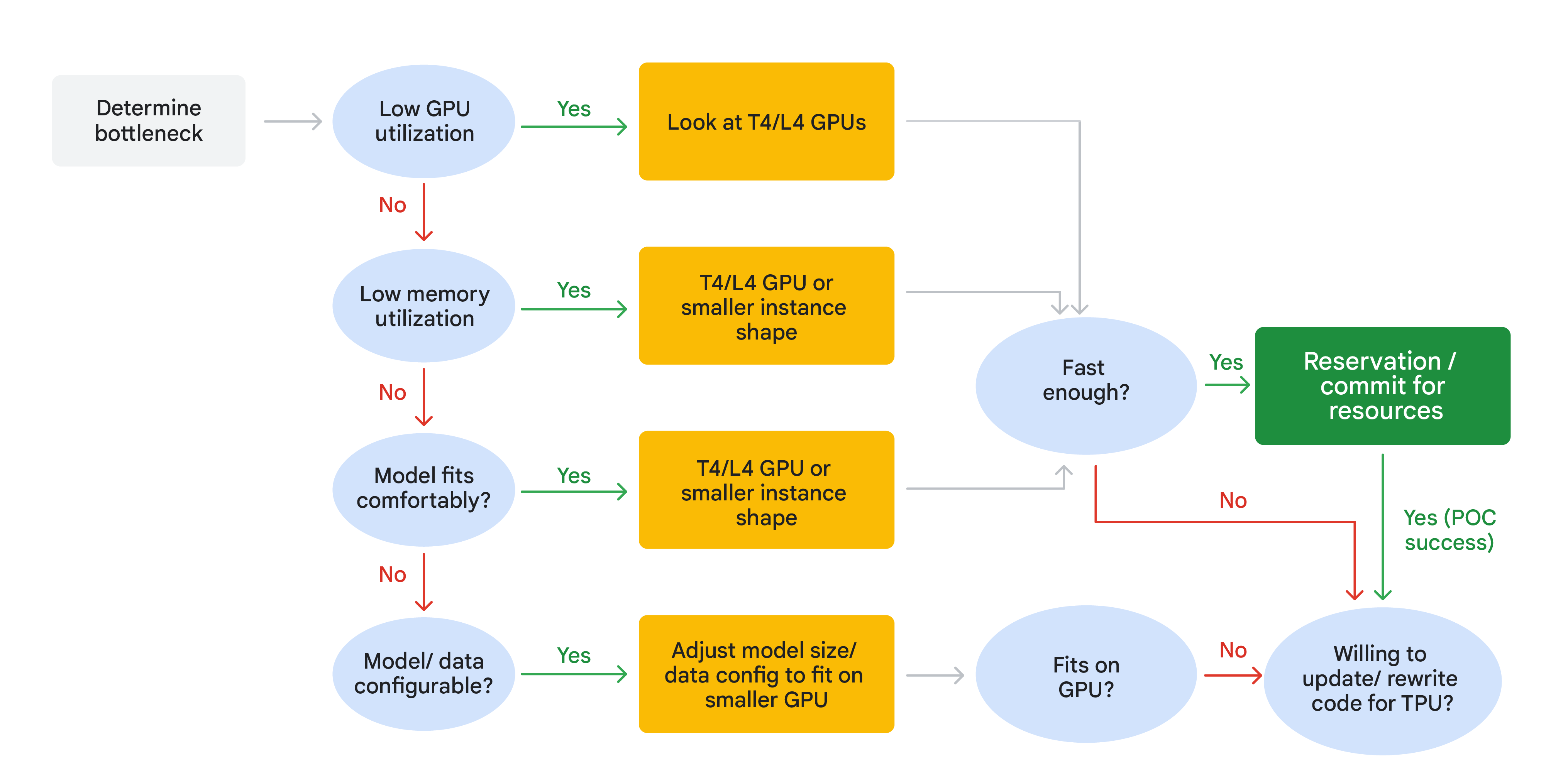
• Start by identifying the bottleneck.
• Low GPU or memory utilization = over-provisioning → move parts of the workload to cheaper T4/L4 GPUs or smaller instance shapes, even if the model fits comfortably on the A100.
• Model struggles to fit → adjust model size or data config to better use the existing high-end GPU.
• After adjusting, ask "fast enough?" If yes → commit to reservations for long-term savings (POC success).
• If not, and you can update/rewrite code → consider migrating to TPUs (e.g. TPU v5e) for potentially large gains.
• If a TPU migration is not feasible → re-check whether the model genuinely fits on GPU, and either optimize further or simplify the model.

Optimizing GPU training time

This tree targets training time by chasing the bottleneck through the data, hardware, network, and code layers in turn.

GPU training-time decision tree - test data loading, then GPU utilization, then network latency, then code; after each fix ask 'fast enough?' and either reserve resources or consider a TPU rewrite.

#NumbersTraining-time flow

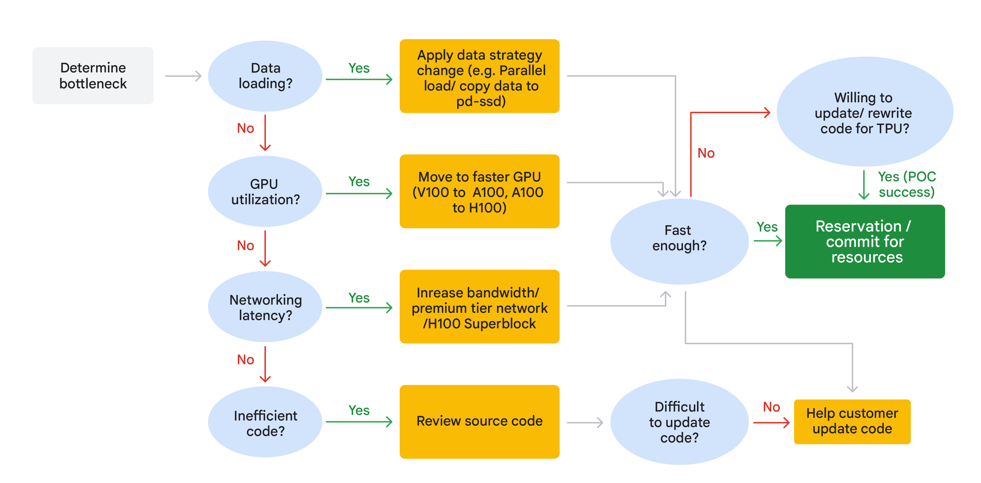
• Data loading the bottleneck? → apply a data strategy change: parallel loading, or copy data to faster storage like a pd-ssd.
• GPU utilization low? → move to a faster GPU (V100 → A100, or A100 → H100).
• Network latency high? → increase bandwidth / use premium-tier networking, or an H100 Superblock for better data transfer (matters most in distributed setups).
• None of the above? → the problem is likely inefficient code; review the source for optimization opportunities. If code is hard to update, help the customer update it.
• After each fix, ask "fast enough?" If yes → reserve/commit resources (POC success). If not and code updates are feasible → consider updating/rewriting for a TPU.

Recap

#NumbersGPU decision - key takeaways

• Differentiate the task first - training/fine-tuning vs inferencing is always the most critical branch.
• Scale matters immensely - model size, number of VMs, and total GPU count drive the hardware tier.
• Latency is a deciding factor - if the app needs rapid responses or quick iteration, prioritize high-speed interconnects like NVLink.
• T4/L4 - versatile and cost-effective across smaller to medium-scale training and inference.
• H100/A100/V100 - the powerhouses; when you hit limits of scale, memory, and latency, these NVLink-capable GPUs handle the most intensive tasks.
• Always validate performance with your actual workload before committing.

For the exam-facing angle - attaching GPUs to VMs, quota, and zonal availability - see GPUs & TPUs.